Introduction to the rbrsa package
The rbrsa package facilitates programmatic access to
Turkish banking sector data from the Turkish Banking Regulation and
Supervision Agency (BRSA, known as BDDK in Turkish). The package
provides R users with a clean interface to fetch monthly and quarterly
banking statistics, financial reports, and sectoral indicators directly
from BRSA’s official APIs. This vignette demonstrates a complete
workflow: from discovering available data to fetching it and performing
a basic analysis.
Installation and Setup
# Install from CRAN
install.packages("rbrsa")

# Or install the development version from GitHub
# install.packages("pak")
pak.::pkg_install("obakis/rbrsa")Part 1: Discovering Available Data
Before requesting data, it’s useful to explore what tables and
banking groups are available from BDDK’s two main portals.
Both portals are official sources, but they organize the data
differently: The Monthly
Bulletin Portal provides high-level, summary reports designed for
general consumption and quick overviews of monthly trends without any
geographic coverage. The Finturk Data System
provides granular, detailed data, including statistics broken down by
province, whereas the standard Monthly Bulletin offers national-level
aggregates.
Important note: Currently, only a single
grup_kod can be specified per request. The underlying BDDK
API supports multiple grup_kod codes, and this
functionality will be added in a future version.
Monthly Bulletin Tables
Monthly Bulletin provides high-level, national aggregate statistics.
# List available tables in the Monthly Bulletin
bulletin_tables <- list_tables("bddk", lang="en")
#> Available tables for bddk data:
#>  Table_No                            Title
#>         1                    Balance Sheet
#>         2                  Profit and Loss
#>         3                            Loans
#>         4                   Consumer Loans
#>         5       Sectoral Loan Distribution
#>         6                        SME Loans
#>         7 Syndication Securitization Loans
#>         8                       Securities
#>         9                 Deposits by Type
#>        10             Deposits by Maturity
#>        11               Liquidity Position
#>        12                 Capital Adequacy
#>        13        Foreign Currency Position
#>        14   Off-Balance Sheet Transactions
#>        15                           Ratios
#>        16                Other Information
#>        17            Foreign Branch Ratios
head(bulletin_tables)
#>   Table_No                      Title
#> 1        1              Balance Sheet
#> 2        2            Profit and Loss
#> 3        3                      Loans
#> 4        4             Consumer Loans
#> 5        5 Sectoral Loan Distribution
#> 6        6                  SME Loans

# List available banking groups for the Monthly Bulletin
bulletin_groups <- list_groups("bddk", lang="en")
#> Available banking groups for bddk data:
#>  Group_Code                             Name
#>       10001                     Sector Total
#>       10002                    Deposit Banks
#>       10008       Deposit - Domestic Private
#>       10009                 Deposit - Public
#>       10010                Deposit - Foreign
#>       10003              Participation Banks
#>       10004 Development and Investment Banks
#>       10005           Domestic Private Banks
#>       10006                     Public Banks
#>       10007                    Foreign Banks
head(bulletin_groups)
#>   Group_Code                       Name
#> 1      10001               Sector Total
#> 2      10002              Deposit Banks
#> 3      10008 Deposit - Domestic Private
#> 4      10009           Deposit - Public
#> 5      10010          Deposit - Foreign
#> 6      10003        Participation Banks
Finturk Tables
Finturk system provides more granular data, including provincial breakdowns.
# List available tables in Finturk
finturk_tables <- list_tables("finturk", lang="en")
#> Available tables for finturk data:
#>  Table_No                                        Title
#>         1                          Loans (Thousand TL)
#>         2                       Deposits (Thousand TL)
#>         3                 Retail Banking (Thousand TL)
#>         4        Selected Sectoral Loans (Thousand TL)
#>         5                                   Ratios (%)
#>         6 Branches and Distribution by Population (TL)
#>         7   Gold Loans and Gold Deposits (Thousand TL)
finturk_tables
#>   Table_No                                        Title
#> 1        1                          Loans (Thousand TL)
#> 2        2                       Deposits (Thousand TL)
#> 3        3                 Retail Banking (Thousand TL)
#> 4        4        Selected Sectoral Loans (Thousand TL)
#> 5        5                                   Ratios (%)
#> 6        6 Branches and Distribution by Population (TL)
#> 7        7   Gold Loans and Gold Deposits (Thousand TL)

# List available banking groups for Finturk
finturk_groups <- list_groups("finturk", lang="en")
#> Available banking groups for finturk data:
#>  Group_Code                             Name
#>       10001                     Sector Total
#>       10002                    Deposit Banks
#>       10003 Development and Investment Banks
#>       10004              Participation Banks
#>       10005                    Foreign Banks
#>       10006                     Public Banks
#>       10007           Domestic Private Banks
finturk_groups
#>   Group_Code                             Name
#> 1      10001                     Sector Total
#> 2      10002                    Deposit Banks
#> 3      10003 Development and Investment Banks
#> 4      10004              Participation Banks
#> 5      10005                    Foreign Banks
#> 6      10006                     Public Banks
#> 7      10007           Domestic Private Banks

# List of cities for Finturk
cities <- list_cities()
#> Available cities for Finturk quarterly data
#> Use license plate number (plaka) in fetch_finturk functions:
#> Valid values: 0 (HEPSI/ALL), 1-81, 999 (YURT DISI/ABROAD)
#>  plaka             il
#>      0          HEPSİ
#>      1          ADANA
#>      2       ADIYAMAN
#>      3 AFYONKARAHİSAR
#>      4           AĞRI
#>      5         AMASYA
#>      6         ANKARA
#>      7        ANTALYA
#>      8         ARTVİN
#>      9          AYDIN
#>     10      BALIKESİR
#>     11        BİLECİK
#>     12         BİNGÖL
#>     13         BİTLİS
#>     14           BOLU
#>     15         BURDUR
#>     16          BURSA
#>     17      ÇANAKKALE
#>     18        ÇANKIRI
#>     19          ÇORUM
#>     20        DENİZLİ
#>     21     DİYARBAKIR
#>     22         EDİRNE
#>     23         ELAZIĞ
#>     24       ERZİNCAN
#>     25        ERZURUM
#>     26      ESKİŞEHİR
#>     27      GAZİANTEP
#>     28        GİRESUN
#>     29      GÜMÜŞHANE
#>     30        HAKKARİ
#>     31          HATAY
#>     32        ISPARTA
#>     33         MERSİN
#>     34       İSTANBUL
#>     35          İZMİR
#>     36           KARS
#>     37      KASTAMONU
#>     38        KAYSERİ
#>     39     KIRKLARELİ
#>     40       KIRŞEHİR
#>     41        KOCAELİ
#>     42          KONYA
#>     43        KÜTAHYA
#>     44        MALATYA
#>     45         MANİSA
#>     46  KAHRAMANMARAŞ
#>     47         MARDİN
#>     48          MUĞLA
#>     49            MUŞ
#>     50       NEVŞEHİR
#>     51          NİĞDE
#>     52           ORDU
#>     53           RİZE
#>     54        SAKARYA
#>     55         SAMSUN
#>     56          SİİRT
#>     57          SİNOP
#>     58          SİVAS
#>     59       TEKİRDAĞ
#>     60          TOKAT
#>     61        TRABZON
#>     62        TUNCELİ
#>     63      ŞANLIURFA
#>     64           UŞAK
#>     65            VAN
#>     66         YOZGAT
#>     67      ZONGULDAK
#>     68        AKSARAY
#>     69        BAYBURT
#>     70        KARAMAN
#>     71      KIRIKKALE
#>     72         BATMAN
#>     73         ŞIRNAK
#>     74         BARTIN
#>     75        ARDAHAN
#>     76          IĞDIR
#>     77         YALOVA
#>     78        KARABÜK
#>     79          KİLİS
#>     80       OSMANİYE
#>     81          DÜZCE
#>    999      YURT DIŞI
head(cities)
#>   plaka             il
#> 1     0          HEPSİ
#> 2     1          ADANA
#> 3     2       ADIYAMAN
#> 4     3 AFYONKARAHİSAR
#> 5     4           AĞRI
#> 6     5         AMASYA
Part 2: Fetching Monthly Bulletin Data
Let’s fetch “Table 4: Consumer Loans” for public banks
(grup_kod = 10006) between January 2020 and December
2020.
my_dat <- fetch_bddk(
  start_year = 2020,
  start_month = 1,
  end_year = 2020,
  end_month = 12,
  table_no = 4,
  grup_kod = 10001,
  verbose=TRUE
)
#> Fetching table 4 for 12 months: 2020-01 to 2020-12
#> [1/12] 2020-01... 41 rows
#> [2/12] 2020-02... 41 rows
#> [3/12] 2020-03... 41 rows
#> [4/12] 2020-04... 41 rows
#> [5/12] 2020-05... 41 rows
#> [6/12] 2020-06... 41 rows
#> [7/12] 2020-07... 41 rows
#> [8/12] 2020-08... 41 rows
#> [9/12] 2020-09... 41 rows
#> [10/12] 2020-10... 41 rows
#> [11/12] 2020-11... 41 rows
#> [12/12] 2020-12... 41 rows
# Examine the structure of the returned data
cat("Dimensions:", dim(my_dat), "\n")
#> Dimensions: 492 10
colnames(my_dat)
#>  [1] "group_name" "BasitSira"  "Ad"         "BasitFont"  "TRY"
#>  [6] "FX"         "Total"      "grup_kod"   "period"     "currency"
head(my_dat)
#>       group_name BasitSira                                    Ad BasitFont
#> 1 Banking Sector         1                Consumer Loans (2+3+4)      bold
#> 2 Banking Sector         2              Consumer Loans - Housing
#> 3 Banking Sector         3              Consumer Loans - Vehicle
#> 4 Banking Sector         4     Consumer Loans - Personal Finance
#> 5 Banking Sector         5   Consumer Loans - Fx Indexed (6+7+8)      bold
#> 6 Banking Sector         6 Consumer Loans - Housing (Fx Indexed)
#>      TRY FX  Total grup_kod  period currency
#> 1 480482 82 480564    10001 2020-01       TL
#> 2 202648 46 202694    10001 2020-01       TL
#> 3   6979  0   6979    10001 2020-01       TL
#> 4 270855 36 270892    10001 2020-01       TL
#> 5     65  0     65    10001 2020-01       TL
#> 6     55  0     55    10001 2020-01       TL
## To save the results:
# temp_file <- tempfile() # filename should be without extension
# save_data(my_dat, temp_file, format = "csv")
Let’s compare “Consumer Loans - Housing” and “Consumer Loans - Personal Finance” over time.
library(dplyr)
library(ggplot2)
colnames(my_dat)
#>  [1] "group_name" "BasitSira"  "Ad"         "BasitFont"  "TRY"
#>  [6] "FX"         "Total"      "grup_kod"   "period"     "currency"
cols = c("Consumer Loans - Housing","Consumer Loans - Personal Finance")
p = my_dat |>
  select(Ad,TRY,period) |>
  filter(Ad %in% cols) |>
  mutate(date=as.Date(paste0(period, "-01"))) |>
  ggplot(aes(x=date, y=TRY, color=Ad, group=Ad, shape=Ad)) +
  geom_line(linewidth = 1) +
  geom_point(size = 2.4, alpha = 0.7) +
  scale_x_date(
    date_breaks = "2 months",      # Show tick every 3 months
    date_labels = "%b %Y",         # Format as "Jan 2020"
    expand = c(0.01, 0)           # Reduce padding
  ) +
  scale_y_continuous(
    labels = scales::comma       # Format numbers with commas
  ) +
  labs(
    title = "Consumer Loans Trends, Jan 2020-Dec 2020 (TRY)",
    subtitle = "Monthly data for Housing vs Personal Finance loans",
    x = "",
    y = ""
  ) +
  theme_minimal() +
theme(
    legend.position = "bottom",  # This moves the legend to the bottom
    axis.text.x = element_text(angle = 45, hjust = 1),
    plot.title = element_text(face = "bold", size = 14),
  )
p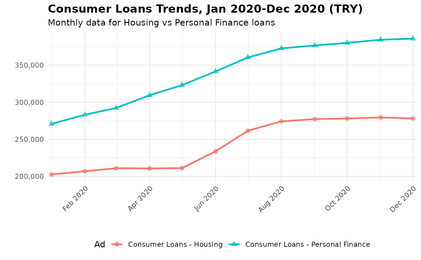
Part 3: Fetching Granular Finturk Data
Now let’s explore the more detailed Finturk data. We’ll fetch “Table
2: Deposits” for all banks (grup_kod = 10001), all
provinces over 2023 and 2024.
my_dat2 <- fetch_finturk(
  start_year = 2023,
  start_month = 3,
  end_year = 2024,
  end_month = 12,
  table_no = 2,
  grup_kod = 10001,
  il=0,
  verbose=FALSE
)
# Examine the structure of the returned data
cat("Dimensions:", dim(my_dat2), "\n")
#> Dimensions: 656 15
colnames(my_dat2)
#>  [1] "grup_kod"                "Yıl"
#>  [3] "Ay"                      "il_adi"
#>  [5] "Grup"                    "Tasarruf Mevduatı"
#>  [7] "Tasarruf Mevduatı (TL)"  "Tasarruf Mevduatı (DTH)"
#>  [9] "Diğer Mevduat"           "Diğer Mevduat (TL)"
#> [11] "Diğer Mevduat (DTH)"     "Toplam Mevduat"
#> [13] "plaka"                   "period"
#> [15] "table_no"
head(my_dat2)
#>   grup_kod  Yıl Ay         il_adi   Grup Tasarruf Mevduatı
#> 1    10001 2023  3          ADANA SEKTÖR         101555827
#> 2    10001 2023  3       ADIYAMAN SEKTÖR          14189512
#> 3    10001 2023  3 AFYONKARAHİSAR SEKTÖR          26182581
#> 4    10001 2023  3           AĞRI SEKTÖR           4541209
#> 5    10001 2023  3        AKSARAY SEKTÖR          22535449
#> 6    10001 2023  3         AMASYA SEKTÖR           9456856
#>   Tasarruf Mevduatı (TL) Tasarruf Mevduatı (DTH) Diğer Mevduat
#> 1               68165445                33390382      40948954
#> 2                8769470                 5420042       4133270
#> 3               13630002                12552579       7218373
#> 4                2860903                 1680306       1495488
#> 5               10411079                12124370       4662855
#> 6                5505734                 3951122       1956146
#>   Diğer Mevduat (TL) Diğer Mevduat (DTH) Toplam Mevduat plaka  period table_no
#> 1           29321746            11627208      142504781     1 2023-03        2
#> 2            3422143              711127       18322782     2 2023-03        2
#> 3            5476164             1742209       33400954     3 2023-03        2
#> 4            1246086              249402        6036697     4 2023-03        2
#> 5            3259852             1403003       27198304    68 2023-03        2
#> 6            1588133              368013       11413002     5 2023-03        2
## To save the results:
# temp_file <- tempfile() # filename should be without extension
# save_data(my_dat, temp_file, format = "csv")
Finturk data includes a province column (il). Let’s
examine the share of selected provinces in total deposits ove 2020-2024
period.
sel_cities =c("ADANA","MALATYA","MUGLA","KAYSERI")
cols = c("il_adi", "period","Toplam Mevduat")
lookup <- c(city="il_adi", deposit="Toplam Mevduat")
p2 = my_dat2[,cols] |>
  rename(all_of(lookup)) |>
  mutate(date=as.Date(paste0(period, "-01"))) |>
  mutate(.by=period, sh = 100*deposit/sum(deposit, na.rm=TRUE)) |>
  filter( city %in% sel_cities) |>
    ggplot(aes(x=date, y=sh, color=city, group=city, shape=city)) +
  geom_line(linewidth = 1) +
  geom_point(size = 2.4, alpha = 0.7) +
  scale_x_date(
    date_breaks = "3 months",      # Show tick every 3 months
    date_labels = "%b %Y",         # Format as "Jan 2020"
    expand = c(0.01, 0)           # Reduce padding
  ) +
  labs(
    title = "Share of Selected Provinces in Deposits, 2020-2023 (TRY)",
    x = "",
    y = ""
  ) +
  theme_minimal() +
theme(
    legend.position = "bottom",  # This moves the legend to the bottom
    axis.text.x = element_text(angle = 45, hjust = 1),
    plot.title = element_text(face = "bold", size = 14),
  )
p2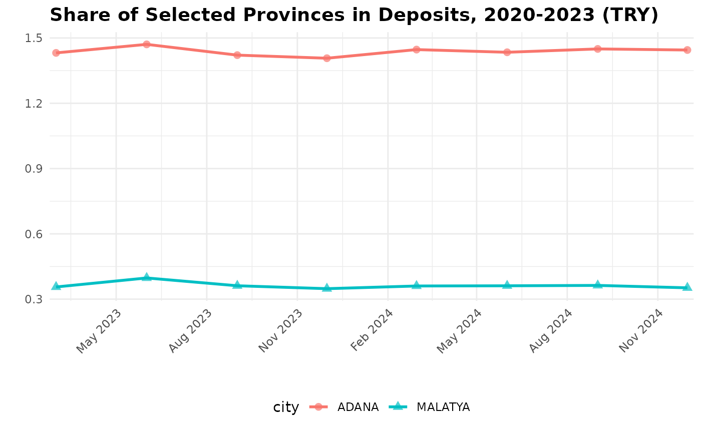
Part 4: Saving Your Results
The save_data() function allows you to export results in
various formats for use in other tools.
# Save to different formats. file name must be without extension
save_data(my_dat, "filename_you_prefer", format = "csv")
save_data(my_dat, "filename_you_prefer", format = "rds")
save_data(my_dat, "filename_you_prefer", format = "xlsx")


temp_file <- tempfile()
save_data(my_dat, temp_file, format = "csv")
message("Data saved to:", temp_file)
Next Steps
This vignette demonstrated the basic workflow of the
rbrs package. To learn more:
- Explore all functions in the package reference: https://obakis.github.io/rbrsa/reference/
- Try different tables and banking groups using
list_tables()andlist_groups(). - Check out the
pybrsapackage (https://github.com/obakis/pybrsa) for similar functionality in Python. (UNDER CONSTRUCTION)
For more detailed function references and advanced usage, visit the complete package documentation at https://obakis.github.io/rbrsa/